Module 3
Ocean Carbon Storage and Acidification
By Prof. Allison Jacobel
Middlebury College, Department of Earth and Climate Sciences
SUMMARY
This module guides students through an examination of how Earth scientists use marine sediments to reconstruct changes in Earth’s climate and the carbon cycle. In Part A, students learn about ocean acidification using modern observations of the atmosphere and ocean, building on previous modules. In Part B, students examine the geologic record of ocean acidification using sediment cores that capture the Paleocene-Eocene Thermal Maximum (PETM). In Part C, students evaluate model projections from the IPCC to compare modern and future carbon cycle change to the PETM and articulate an argument that we need to stop emitting carbon as soon as possible.
The overarching questions the module helps students answer are:
How does anthropogenic carbon release impact the oceans?
How do scientists reconstruct past climate and carbon cycle change?
How does the current rate of carbon release compare to an extreme event in Earth’s history?
These questions correspond with Next-Generation Science Standards (NGSS) HS-ESS2-2:
Analyze geoscience data to make the claim that one change to Earth’s surface can create feedbacks that cause changes to other Earth systems.
and HS-ESS3-5:
Analyze geoscience data and the results from global climate models to make an evidence-based forecast of the current rate of global or regional climate change and associated impacts to Earth systems.
Module Strengths
This activity has been designed using a modified Project EDDIE (Environmental Data-Driven Inquiry and Exploration) module framework. The module is focused on giving students an opportunity to use large, real-world data sets to improve their quantitative reasoning through self-directed inquiry.
This module uses published data sets that are fundamental to our understanding of Earth's carbon cycle history. The module guides students through hands-on, descriptive, and numerical analysis of data sets. The module structure requires students to work independently and collaboratively, and provides opportunities for self-assessment, peer check-in, and instructor evaluation.
What Success Looks Like
By the end of the module students should be able to:
Describe how sediment cores can be analyzed to obtain information about Earth’s climate history.
Understand the consequences of anthropogenic carbon release for calcareous organisms in the ocean.
Evaluate rates of change to determine that the current rate of anthropogenic CO2 release is higher than during a major mass extinction.
Articulate an argument for reducing carbon emissions.
Context for Use
This module was designed for use as part of a 12th grade IB course on ‘Environmental Systems and Societies’. The module should take approximately 100 minutes total (1-2 class periods) to complete, including the presentation of the module PowerPoint. Module Activities A and B are designed to be completed individually; Activity C should be completed and presented in collaborative teams.
MODULE
PART A – MODERN OBSERVATIONS
As you learned in the pre-module lecture, changes in the concentration (or partial pressure) of CO2 in the atmosphere have an impact on the concentration of CO2 that is dissolved in the surface ocean. When CO2 is released (through the burning of fossil fuels) it causes the pH of the surface ocean to change.
1. If the CO2 content of the surface ocean is increased, how might we expect the pH of the water to change? Recall that CO2 reacts with water to form H2CO3 (carbonic acid), and can further ‘disassociate’ into HCO3- (bicarbonate) and CO32- (carbonic acid) plus H+. Also recall the definition of pH.

Figure 1. Carbonate system equations
2. Below is a diagram that should be partly familiar to you from a previous module. The red line is the ‘Keeling Curve’ which represents measurements of atmospheric CO2 from 1958 to present. The green line on the plot shows the concentration of CO2 in the surface ocean over the same time interval. Why does the green line follow the red line?

Figure 2. Measurements of atmospheric and surface ocean CO2 (y-axis at left) and pH (y-axis at right) from the long-term monitoring stations in the Hawaiian Islands.
3. The blue line in the figure depicts measurements of surface ocean pH over the same time interval. Note that the axis that corresponds to this data set is on the right-hand y-axis. Why does the pH go down over this interval as CO2 goes up?
4. Remind yourself of what ‘log’ means in math. If the pH changes from 8 to 7 (bigger than the current magnitude of change) what change in H+ concentration does that represent?
Calcareous organisms, those that build shells out of calcium carbonate, are sensitive to the pH of the ocean. As the pH of the ocean is lowered (more acidic), there is less available carbonate ion and bicarbonate for them to build their shells. Science journalist Elizabeth Kolbert draws an analogy between the loss of carbonate ion caused by ocean acidification a stealing of the ‘bricks’ that calcareous organisms use to build their ‘homes’. When ocean conditions become too acidic organisms will have trouble forming their shells and may actually begin to lose calcite and dissolve.

Figure 3. Pteropod image from ColdWater Science.
Pteropods or sea butterflies (Fig. 3 at left) are calcareous organisms that are abundant in the modern oceans. Below you can see images of pteropods that have been exposed to acidic waters. Note how the shell changes as the pH is reduced. The frosting and pitting you see is due to loss of CaCO3. This is qualitative evidence of acidification affecting shells. If the pH drops low enough it will kill the organism, further decreases may cause the shell to dissolve completely (Fig. 4 below).
Although qualitative evidence can be visually compelling, scientists often wish to quantify processes to describe rates of change over time or compare conditions at different sites in an absolute way. One way to do this with calcareous organisms is to take measurements of shell weights and normalize (or divide) them by the size of the shell. This allows scientists to control for shell size and quantitatively compare the density (mass/area) of different shells. More dense shells have more calcite, less dense shells have less calcite and indicate greater dissolution. Thus, shell density is a quantitative metric that we can use to describe the effects of low pH across a single species.

Figure 4. Pteropods exposed to reduced pH (acidic) conditions. Image from the Seattle Times.
Although qualitative evidence can be visually compelling, scientists often wish to quantify processes to describe rates of change over time or compare conditions at different sites in an absolute way. One way to do this with calcareous organisms is to take measurements of shell weights and normalize (or divide) them by the size of the shell. This allows scientists to control for shell size and quantitatively compare the density (mass/area) of different shells. More dense shells have more calcite, less dense shells have less calcite and indicate greater dissolution. Thus, shell density is a quantitative metric that we can use to describe the effects of low pH across a single species.

Figure 5. Graphic from Osbourne et al., 2020 showing changes in foraminifera density through time. Panel a depicts a foraminifera - a microscopic protist that lives in the surface of the ocean. Panels b and c show cross sections through the shells of foraminifera with b indicating thick, dense calcite as observed in a sample from 1900 and c indicating thinned calcite observed in the year 2000.
5. Examine Figure 5 at left from a paper by Osbourne et al., 2020. The graph shows changes in shell densities of calcareous organism called foraminifera. What time period does the study cover?
6. What is the general trend in shell density (ANSW – area normalized shell weight) over that interval?
7. Is the rate of change constant over the study interval?
8. Does the direction of the trend match your expectations based on the Keeling Curve above? Why or why not?
9. Does the slope of the trend match your expectations based on the Keeling Curve?
10. Why might biological organisms show a non-linear response to changes in pH?
PART B – OBSERVATIONS OF THE PALEOCENE-EOCENE THERMAL MAXIMUM (PETM)
The kinds of shell density measurements described above, for modern shells, can also be used on marine sediment cores to quantify changes in ocean pH in Earth’s history. Quantifying these changes helps us understand how much pH change might occur for a given change in atmospheric pCO2. These kinds of estimates are important for predicting how bad ocean acidification might get in the near future, and 100 years or more from now.
In addition to observing shell densities, scientists also have other ways of determining whether changes in ocean pH have occurred. For example, they might observe changes in the color of sediments deposited on the seafloor. Sediments that are whiter in color often indicate that the shells of calcareous organisms (like pteropods or foraminifera) were abundant during those times, whereas sediments that are darker in color (think dark like organic-rich topsoil from a garden or compost) may have higher organic matter contents or be derived from dark-colored terrestrial rocks.

Figure 6. Dr. James Zachos holding a core that covers the PETM. Photo by National Geographic.
At right is a (delightfully serious) picture of Dr. James Zachos of the University of California Santa Barbara standing with a (replica) core that covers an interval of geologic time known as the Paleocene-Eocene Thermal Maximum or (PETM). The PETM was a mass extinction event (one of the ‘Big Five’) that occurred 55 Ma ago (about 10 Ma after the non-avian dinosaurs went extinct).
1. Examine the sediment core Dr. Zachos is holding. Describe the relative carbonate composition of the core starting at the bottom (oldest) and moving towards the top? Pay particular attention to relative rates of change.
2. Based on what you have learned about the conditions under which calcium carbonate is preserved/dissolved, what direction do you think ocean pH went at the time of the PETM?
3. Do some research online. What organisms went extinct at the PETM? Were there any patterns in extinction? Habitats that were hardest hit? Types of organisms?
4. Do you see evidence that ocean pH ‘recovered’ after the PETM? Explain.
5. Using sophisticated geochemical techniques (isotopes of boron and carbon measured on foraminifera) scientists have determined that during the PETM ocean pH changed between 0.27 - 0.36 units as a consequence of the release of 10,200 Pg (peta grams) of carbon was over a 50 kyr interval, because of massive volcanic eruptions. One Peta gram is the same as a Gigaton or one billion tons. Calculate the annual release rate of carbon at the PETM. Hint: Your answer should have units of Pg/yr.
6. The rate of CO2 emissions as of 2022 is 37 Pg/yr. How does this compare to the rate of release at the PETM mass extinction event?
PART C – IPCC PROJECTIONS AND THE CASE FOR REDUCING CARBON EMISSIONS
As we discussed in class, the Intergovernmental Panel on Climate Change (IPCC) puts out regular reports that include predictions for Earth’s future (surface temperature, sea level, ocean pH etc.) based on different emissions scenarios.
From the five IPCC Scenarios choose one for your group to focus on. You will compare your results to other groups who chose a different scenario.

Figure 7. Graph of annual CO2 emission rate for the IPCC SSP scenarios
First, remind yourself of the characteristics of your SSP. Then, using the data supplied by the International Institute for Applied Systems Analysis at left (Figure 6) and below (Table 1) examine your SSP with respect to CO2 emission rate per year.
1. What does your SSP ‘predict’ annual emissions will be in 2050? What about in 2100? How do these values compare to the annual release at the PETM?
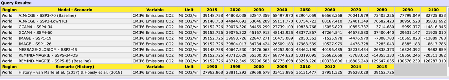
Table 1. Annual CO2 emission rate for the IPCC SSP scenarios. Note the units are in megatons of CO2/yr. 1 Mt = 0.001 Pg
2. Examine the graphs of SSP changes to sea surface temperature (SST) estimates and pH below (Fig 8). What is the magnitude of warming simulated for your SSP in 2050? In 2100?
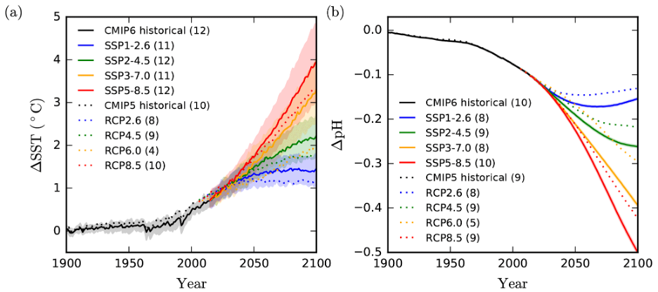
Figure 8. IPCC predictions from Kwiatkowski et al. 2020 for the change in a. sea surface temperature (SST) and b. pH under different SSP scenarios.
3. What is the estimated pH change for your SSP? How does this compare to the PETM (see B5 above)?
4. Compare your results with groups that examined different SSPs.
5. Use your findings and comparisons to the PETM mass extinction to write a short paragraph arguing that every ton of CO2 emission reductions matters. Your argument should include global temperature change, pH changes, and other climate feedbacks.
Module also available as a download from the SERC website at: https://serc.carleton.edu/teachearth/activities/281458.html